Bayes Theorem Calculator

1. Bayes Theorem (Bayes Formula, Bayes Rule)
2. Practical applications of the Bayes Theorem
• Cancer diagnosis
• Drug test
• Quality assurance
• Spam Filtering
3. Base rate fallacy

    Bayes Theorem (Bayes Formula, Bayes Rule)

The Bayes Theorem is named after Reverend Thomas Bayes (1701–1761) whose manuscript reflected his solution to the inverse probability problem: computing the posterior conditional probability of an event given known prior probabilities related to the event and relevant conditions. It was published posthumously with significant contributions by R. Price ^[1] and later rediscovered and extended by Pierre-Simon Laplace in 1774.

In its current form, the Bayes theorem is usually expressed in these two equations:

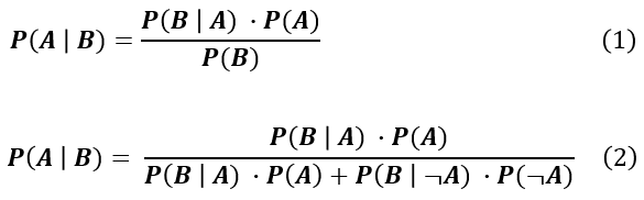
where A and B are events, P() denotes "probability of" and | denotes "conditional on" or "given". Both forms of the Bayes theorem are used in this Bayes calculator.

The first formulation of the Bayes rule can be read like so: the probability of event A given event B is equal to the probability of event B given A times the probability of event A divided by the probability of event B. In statistics P(B|A) is the likelihood of B given A, P(A) is the prior probability of A and P(B) is the marginal probability of B. The alternative formulation (2) is derived from (1) with an expanded form of P(B) in which A and ¬A (not-A) are disjointed (mutually-exclusive) events. This formulation is useful when we do not directly know the unconditional probability P(B).

The Bayes formula has many applications in decision-making theory, quality assurance, spam filtering, etc. This Bayes theorem calculator allows you to explore its implications in any domain. With probability distributions plugged in instead of fixed probabilities it is a cornerstone in the highly controversial field of Bayesian inference (Bayesian statistics).

    Practical applications of the Bayes Theorem

Here we present some practical examples for using the Bayes Rule to make a decision, along with some common pitfalls and limitations which should be observed when applying the Bayes theorem in general.

Cancer diagnosis

A woman comes for a routine breast cancer screening using mammography (radiology screening). On average the mammograph screening has an expected sensitivity of around 92% and expected specificity of 94%. Sensitivity reflects the percentage of correctly identified cancers while specificity reflects the percentage of correctly identified healthy individuals. Their complements reflect the false negative and false positive rate, respectively. We also know that breast cancer incidence in the general women population is 0.089%.

Plugging the numbers in our calculator we can see that the probability that a woman tested at random and having a result positive for cancer is just 1.35%. Quite counter-intuitive, right?

However, the above calculation assumes we know nothing else of the woman or the testing procedure. Let us narrow it down, then. If we also know that the woman is 60 years old and that the prevalence rate for this demographic is 0.351% ^[2] this will result in a new estimate of 5.12% (3.8x higher) for the probability of the patient actually having cancer if the test is positive.

Now, if we also know the test is conducted in the U.S. and consider that the sensitivity of tests performed in the U.S. is 91.8% and the specificity just 83.2% ^[3] we can recalculate with these more accurate numbers and we see that the probability of the woman actually having cancer given a positive result is increased to 16.58% (12.3x increase vs initial) while the chance for her having cancer if the result is negative increased to 0.3572% (47 times! vs initial).

In this example you can see both benefits and drawbacks and limitations in the application of the Bayes rule. First, it is obvious that the test's sensitivity is, by itself, a poor predictor of the likelihood of the woman having breast cancer, which is only natural as this number does not tell us anything about the false positive rate which is a significant factor when the base rate is low. We need to also take into account the specificity, but even with 99% specificity the probability of her actually having cancer after a positive result is just below 1/4 (24.48%), far better than the 83.2% sensitivity that a naive person would ascribe as her probability. Putting the test results against relevant background information is useful in determining the actual probability.

However, it can also be highly misleading if we do not use the correct base rate or specificity and sensitivity rates e.g. if we apply a base rate which is too generic and does not reflect all the information we know about the woman, or if the measurements are flawed / highly uncertain. This is known as the reference class problem and can be a major impediment in the practical usage of the results from a Bayes formula calculator.

For example, if the true incidence of cancer for a group of women with her characteristics is 15% instead of 0.351%, the probability of her actually having cancer after a positive screening result is calculated by the Bayes theorem to be 46.37% which is 3x higher than the highest estimate so far while her chance of having cancer after a negative screening result is 3.61% which is 10 times higher than the highest estimate so far. This is why it is dangerous to apply the Bayes formula in situations in which there is significant uncertainty about the probabilities involved or when they do not fully capture the known data, e.g. because population-level data is not available.

Drug test

Let us say a drug test is 99.5% accurate in correctly identifying if a drug was used in the past 6 hours. It also gives a negative result in 99% of tested non-users. Given that the usage of this drug in the general population is a mere 2%, if a person tests positive for the drug, what is the likelihood of them actually being drugged? Using this Bayes Rule Calculator you can see that the probability is just over 67%, much smaller than the tool's accuracy reading would suggest.

Of course, similar to the above example, this calculation only holds if we know nothing else about the tested person. However, if we know that he is part of a high-risk demographic (30% prevalence) and has also shown erratic behavior the posterior probability is then 97.71% or higher: much closer to the naively expected accuracy. However, if we also know that among such demographics the test has a lower specificity of 80% (i.e. due to it picking up on use which happened 12h or 24h before the test) then the calculator will output only 68.07% probability, demonstrating once again that the outcome of the Bayes formula calculation can be highly sensitive to the accuracy of the entered probabilities.

Quality assurance

The Bayes theorem can be useful in a QA scenario. If we have 4 machines in a factory and we have observed that machine A is very reliable with rate of products below the QA threshold of 1%, machine B is less reliable with a rate of 4%, machine C has a defective products rate of 5% and, finally, machine D: 10%. If we know that A produces 35% of all products, B: 30%, C: 15% and D: 20%, what is the probability that a given defective product came from machine A?

In this case the overall prevalence of products from machine A is 0.35. P(failed QA|produced by machine A) is 1% and P(failed QA|¬produced by machine A) is the sum of the failure rates of the other 3 machines times their proportion of the total output, or P(failed QA|¬produced by machine A) = 0.30 x 0.04 + 0.15 x 0.05 + 0.2 x 0.1 = 0.0395. Thus, if the product failed QA it is 12% likely that it came from machine A, as opposed to the average of 35% of overall production.

Similarly to the other examples, the validity of the calculations depends on the validity of the input. If past machine behavior is not predictive of future machine behavior for some reason, then the calculations using the Bayes Theorem may be arbitrarily off, e.g. if machine A suddenly starts producing 100% defective products due to a major malfunction (in which case if a product fails QA it has a whopping 93% chance of being produced by machine A!).

Spam Filtering

Let us say that we have a spam filter trained with data in which the prevalence of emails with the word "discount" is 1%. Furthermore, it is able to generally identify spam emails with 98% sensitivity (2% false negative rate) and 99.6% specificity (0.4% false positive rate). If the filter is given an email that it identifies as spam, how likely is it that it contains "discount"? In this case, which is equivalent to the breast cancer one, it is obvious that it is all about the base rate and that both sensitivity and specificity say nothing of it. The likelihood that the so-identified email contains the word "discount" can be calculated with a Bayes rule calculator to be only 4.81%.

Perhaps a more interesting question is how many emails that will not be detected as spam contain the word "discount". The answer is just 0.98%, way lower than the general prevalence. Of course, the so-calculated conditional probability will be off if in the meantime spam changed and our filter is in fact doing worse than previously, or if the prevalence of the word "discount" has changed, etc.

    Base rate fallacy

Cases of base rate neglect or base rate bias are classical ones where the application of the Bayes rule can help avoid an error. The fallacy states that if presented with related base rate information (general information) and specific information (pertaining only to the case at hand, e.g. a test result), the mind tends to ignore the former and focus on the latter. The well-known example is similar to the drug test example above: even with test which correctly identifies drunk drivers 100% of the time, if it also has a false positive rate of 5% for non-drunks and the rate of drunks to non-drunks is very small (e.g. 1 in 999), then a positive result from a test during a random stop means there is only 1.96% probability the person is actually drunk.

The opposite of the base rate fallacy is to apply the wrong base rate, or to believe that a base rate for a certain group applies to a case at hand, when it does not. With the above example, while a randomly selected person from the general population of drivers might have a very low chance of being drunk even after testing positive, if the person was not randomly selected, e.g. he was exhibiting erratic driving, failure to keep to his lane, plus they failed to pass a coordination test and smell of beer, it is no longer appropriate to apply the 1 in 999 base rate as they no longer qualify as a randomly selected member of the whole population of drivers. Rather, they qualify as "most positively drunk"...